
Spatial Metabolomics Resolution Guide: From 100μm to 5μm in Plant Tissue Imaging
The resolution chosen for spatial metabolomics critically impacts result quality. What resolution suits brain tissue or plant roots? Is 20μm sufficient for analyzing glomeruli or seed coats? While higher resolution (smaller values) enables finer tissue segmentation, how substantial are the differences between resolutions? Here, we dissect this using experimental data from rapeseed (Brassica napus).
1. Understanding Resolution in Spatial Metabolomics
In spatial mass spectrometry imaging (MSI), resolution refers to the ionized area size detected by the ion source. For MALDI-MSI (Matrix-Assisted Laser Desorption/Ionization MSI), a laser scans the sample in a grid pattern, sublimating matrix-embedded molecules for detection. Thus, resolution aligns with the laser beam size. Higher resolution (e.g., 5μm) reveals intricate structural details but demands higher costs. Below, we compare results across resolutions.

Spatial metabolome enables metabolite tissue distribution detection by raster scanning
2. How Resolution Impacts Spatial MSI Results
2.1 Sample Overview
Adjacent sections of a rapeseed (diameter: 1.2–2.05 mm; seed coat thickness: 26–28μm) were analyzed at 100μm, 50μm, 20μm, 10μm, and 5μm resolutions, followed by segmentation analysis.

Scanning images and structural schematics of the rapeseed
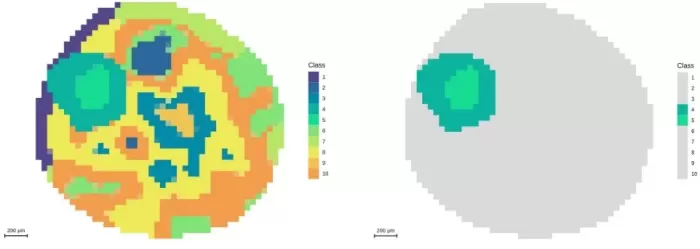
2.2 Imaging at 100μm Resolution
Data: ~400 pixels.
Spatial Distribution (m/z 464.1908): No distinct patterns across tissues.
Segmentation: Roughly identified the embryonic axis (0.7mm diameter) but failed to resolve smaller structures.

Spatial distribution and segmentation maps at 100μm

Segmentation analysis at 100μm resolution and demonstration of embryonic axis regions
2.3 Imaging at 50μm Resolution
Data: ~1,600 pixels.
Spatial Distribution (m/z 464.1908): Specific accumulation in the embryonic axis; minimal patterns elsewhere.
Segmentation: Highlighted embryonic axis gradients but lacked precision for microstructures.

Spatial distribution and segmentation maps at 50μm
Segmentation analysis at 50μm resolution and demonstration of embryonic axis regions
2.4 Imaging at 20μm Resolution
Data: ~10,000 pixels.
Spatial Distribution (m/z 464.1908): Emergence of fine features (e.g., higher metabolite abundance in outer seed coat).
Segmentation: Partially resolved seed coat (26–28μm) but could not distinguish cotyledons.

Spatial distribution and segmentation maps at 20μm

Segmentation analysis at 20μm resolution and demonstration of embryonic axis regions
2.5 Imaging at 10μm Resolution
Data: ~40,000 pixels.
Spatial Distribution (m/z 464.1908): Sharp tissue boundaries (e.g., inner/outer cotyledons) and refined embryonic axis gradients.
Segmentation: Divided seed coat into four sub-regions, aligning better with anatomy.

Spatial distribution and segmentation maps at 10μm

Segmentation analysis at 10μm resolution and demonstration of embryonic axis regions
2.6 Imaging at 5μm Resolution
Data: ~160,000 pixels.
Spatial Distribution (m/z 464.1908): Ultra-fine layers in the seed coat and crisp boundaries between embryonic axis and cotyledons.
Segmentation: Matched anatomical structures with pixel-level accuracy, outperforming 10μm.

Spatial distribution and segmentation maps at 5μm

Segmentation analysis at 5μm resolution and demonstration of embryonic axis regions
3. Resolution Comparison: From Clarity to Cost
3.1 Spatial Distribution Insights
Low Resolutions (100μm, 50μm): Broad patterns, limited detail.
Mid-High Resolutions (20μm–5μm): Progressively enhanced clarity. For a 2mm rapeseed, 20μm (~10,000 pixels) is acceptable, while 5μm (~160,000 pixels) delivers optimal precision.
Recommendation:
- ≥5mm×5mm samples: Use ≤50 μm.
- 2mm×2mm samples: Use ≥20 μm.

Comparative figures of spatial metabolite distributions.
3.2 Segmentation Performance
Embryonic Axis: Detected at ≥50 μm; internal gradients visible at 50 μm.
Seed Coat: Partially resolved at 20 μm; optimally segmented at 5 μm.
Cotyledons: No metabolic divergence observed across resolutions.
Takeaway: 5μm resolution excels for microstructures (e.g., seed coats, glomeruli).
3.3 Guidelines for Microstructures
For features like seed coats (26–28 μm) or glomeruli (20 μm short axis):
Resolution: ≤ feature size.
Pixel Coverage: Feature width/resolution ≥4 (e.g., 5μm resolution for 20 μm structures).
Example: Mouse kidney tubules (30μm diameter) require ≤20μm resolution.

Segmentation of the embryonic axis and seed coat region at different resolutions
4. Resolution Selection Framework
1. General Samples (No Microstructures): Ensure >10,000 pixels (e.g., 50 μm for 5mm×5mm).
2. Samples with Microstructures:
- Minimum Requirement: Resolution < smallest feature.
- Optimal Practice: Feature width/resolution ≥4 (e.g., 5 μm for 20 μm glomeruli).
Final Thoughts: Precision vs Practicality
Higher resolution unlocks unparalleled spatial detail but increases costs. Strategically balance objectives:
- Routine Studies: 20–50μm for most tissues.
- Microstructural Analysis: ≤5μm for pixel-perfect clarity.
By tailoring resolution to biological questions, researchers can map metabolic intricacies with precision.
Next-Generation Omics Solutions:
Proteomics & Metabolomics
Ready to get started? Submit your inquiry or contact us at support-global@metwarebio.com.
