Spatial Metabolomics Data Analysis with Cardinal: A Step-by-Step R Tutorial
Spatial metabolomics not only preserves the qualitative and quantitative strengths of traditional metabolomics but also introduces the ability to precisely localize metabolites within tissues, offering a visual representation of their spatial distribution. This technology provides a significant advantage in tackling the issue of tissue heterogeneity in metabolites. Moreover, the spatial data generated by spatial metabolomics requires unique data processing methods, setting it apart from traditional metabolomics approaches. In the realm of bioinformatics, the R programming language has proven to be a versatile and effective tool for spatial metabolomics data analysis. Among its many packages, Cardinal stands out as a powerful resource for researchers, offering robust data analysis and visualization capabilities. These tools enable scientists to delve deeper into the spatial distribution patterns of metabolites and their biological significance, paving the way for groundbreaking discoveries in the field.
1. Installing and Loading the Cardinal Package
Cardinal can be installed via the BiocManager package. The same function can be used to update Cardinal and other Bioconductor packages. After installation, Cardinal can be loaded using the library() function:
install.packages("BiocManager")
BiocManager::install("Cardinal")
library(Cardinal)
2. Understanding MSImagingExperiment Components
In Cardinal, a spatial metabolomics dataset consists of multiple metadata components in addition to the experimental data itself. These include:
1) Pixel data
2) Feature (m/z) data
3) Imaging intensity data
4) A class encapsulating all these data to represent the entire experiment.
The MSImagingExperiment is a matrix-like container for storing complete MS imaging experiments. Here, "rows" represent m/z features, and "columns" represent pixels.
An MSImagingExperiment object contains the following components:
PositionDataFrame: Accessed via pixelData() for pixel information.
MassDataFrame: Accessed via featureData() for m/z information.
ImageArrayList: Accessed via imageData() for intensity information.
Unlike many software packages designed exclusively for MS imaging analysis, Cardinal is capable of handling multiple datasets simultaneously and integrates all aspects of experimental design and metadata.
2.1 Example Data
The simulateImage() function is used to prepare a sample dataset:
register(SerialParam())
set.seed(2020)
mse <- simulateImage(preset=1, npeaks=10, nruns=2, baseline=1)
mse
Output:
## An object of class 'MSContinuousImagingExperiment'
<3919 feature, 800 pixel> imaging dataset
imageData(1): intensity
featureData(0):
pixelData(1): circle
metadata(1): design
run(2): run0 run1
raster dimensions: 20 x 20
coord(2): x = 1..20, y = 1..20
mass range: 426.5285 to 2044.4400
centroided: FALSE
2.2 pixelData(): Extracting Pixel Information
Pixel data is stored in a PositionDataFrame, a specialized data frame tracking pixel coordinates and experimental run information.
pixelData(mse)
## PositionDataFrame
:run: coord:x coord:y circle
1 run0 1 1 FALSE
2 run0 2 1 FALSE
3 run0 3 1 FALSE
4 run0 4 1 FALSE
5 run0 5 1 FALSE
... ... ... ... ...
796 run1 16 20 FALSE
797 run1 17 20 FALSE
798 run1 18 20 FALSE
799 run1 19 20 FALSE
800 run1 20 20 FALSE
The coord() function extracts pixel coordinates:
coord(mse)
DataFrame with 800 rows and 2 columns
x y
1 1 1
2 2 1
3 3 1
4 4 1
5 5 1
... ... ...
796 16 20
797 17 20
798 18 20
799 19 20
800 20 20
The run() function extracts experimental run data:
run(mse)[1:10]
[1] run0 run0 run0 run0 run0 run0 run0 run0 run0 run0
Levels: run0 run1
2.3 MassDataFrame: m/z Data
Use featureData() to extract m/z information from an MSImagingExperiment:
featureData(mse)
#### MassDataFrame with 3919 rows and 0 columns
:mz:
1 426.529
2 426.699
3 426.870
4 427.041
5 427.211
... ...
3915 2041.17
3916 2041.99
3917 2042.81
3918 2043.62
3919 2044.44
Extract the m/z vector:
mz(mse)[1:10]
[1] 426.5285 426.6991 426.8699 427.0406 427.2115 427.3824 427.5534 427.7245
[9] 427.8956 428.0668
2.4 MSImagingExperiment: Ion Intensity Data
The imageData() function extracts imaging data:
imageData(mse)
## MSContinuousImagingSpectraList of length 1
names(1): intensity
class(1): matrix
dim(1): <3919 x 800>
mem(1): 25.08 MB
Intensity matrices can be accessed via iData() or spectra():
iData(mse, "intensity")
Output:
spectra(mse)[1:5, 1:5]
[,1] [,2] [,3] [,4] [,5]
[1,] 0.9295940 0.9779923 0.9415157 0.9115036 0.8960595
[2,] 1.0087009 1.3108664 1.0928983 1.0243944 1.0706272
[3,] 1.0578001 1.0625834 1.2407371 0.9319758 0.8822412
[4,] 0.8949165 1.1568158 0.9250994 0.9499621 1.0127282
[5,] 1.0660395 1.0123048 1.0291570 0.8999156 1.1126816
3. Data Input and Output with imzML
3.1 Creating Example Files
Cardinal 2 natively supports reading and writing imzML (both "continuous" and "processed" versions) and Analyze 7.5 formats.
set.seed(2020)
tiny <- simulateImage(preset=1, from=500, to=600, dim=c(3,3))
tiny
## An object of class 'MSContinuousImagingExperiment'
<456 feature, 9 pixel> imaging dataset
imageData(1): intensity
featureData(0):
pixelData(1): circle
metadata(1): design
run(1): run0
raster dimensions: 3 x 3
coord(2): x = 1..3, y = 1..3
mass range: 500.0000 to 599.8071
centroided: FALSE
Convert to a "processed" imzML format:
tiny2 <- as(tiny, "MSProcessedImagingExperiment")
tiny2
## An object of class 'MSProcessedImagingExperiment'
<456 feature, 9 pixel> imaging dataset
imageData(1): intensity
featureData(0):
pixelData(1): circle
metadata(1): design
run(1): run0
raster dimensions: 3 x 3
coord(2): x = 1..3, y = 1..3
mass range: 500.0000 to 599.8071
centroided: FALSE
3.2 Reading imzML Files
Use readMSIData() to import imzML files:
The attach.only parameter is used to specify that the intensity data should not be loaded into memory but instead attached as a file-based matrix using the matter package. Starting from Cardinal 2, the default setting for attach.only is TRUE. This approach is more memory-efficient, although some methods may become slower due to file I/O operations. If the mass.range is known, specifying it during the import of imzML data can significantly improve efficiency. This parameter can also be used to pre-filter the data to a smaller mass range.
The resolution parameter is used to define the resolution of the mass-to-charge ratio (m/z), which refers to the interval between each m/z point. Resolution is typically specified in parts per million (ppm), representing the percentage error relative to the m/z value.
path_in <- paste0(path, ".imzML")
tiny2_in <- readMSIData(path2_in, mass.range=c(510,590),attach.only=TRUE,
resolution=100, units="ppm")
tiny2_in
## An object of class 'MSProcessedImagingExperiment'
<1458 feature, 9 pixel> imaging dataset
imageData(1): intensity
featureData(0):
pixelData(0):
metadata(1): parse
run(1): file351679b774db5
raster dimensions: 3 x 3
coord(2): x = 1..3, y = 1..3
mass range: 510.000 to 589.993
centroided: FALSE
4. Visualizing Spatial Metabolomics Data in Cardinal
4.1 plot(): Mass Spectra Visualization
Plot spectra using plot():
plot(mse, pixel=c(211, 611))

Mass Spectra Visualization
4.2 image(): Ion Image Visualization
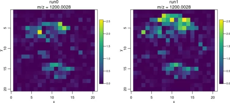
Visualize ion images for specific m/z values:
image(mse, mz=1200)

ion images
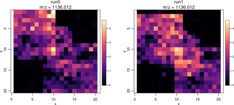
Enhance visualization with color scales:
image(mse2, mz=1136, colorscale=magma)

Enhance visualization of ion images
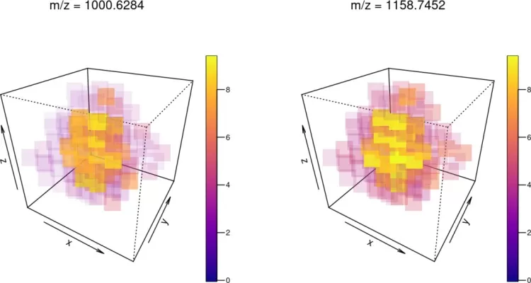
4.3 image3D(): 3D Imaging
Visualize 3D spatial data:
set.seed(1)
mse3d <- simulateImage(preset=9, nruns=7, dim=c(7,7), npeaks=10,
peakheight=c(2,4), representation="centroid")
image3D(mse3d, mz=c(1001, 1159), colorscale=plasma, cex=3, theta=30, phi=30)

3D ion images
4.4 Saving Images
Save plots using R's graphical devices:
pdf_file <- paste0(tempfile(), ".pdf")
pdf(file=pdf_file, width=9, height=4)
image(mse, mz=1200)
dev.off()
In this tutorial, we highlighted key visualization functionalities of the Cardinal package for spatial metabolomics.
Next-Generation Omics Solutions:
Proteomics & Metabolomics
Ready to get started? Submit your inquiry or contact us at support-global@metwarebio.com.


