Data Analysis in Metabolomics Biomarker Research-Biomarker Screening
Metabolomics Biomarker Series Article Catalog:
1. Unlocking Biomarkers: A Guide to Vital Health Indicators
2. Metabolomics and Biomarkers: Unveiling the Secrets of Biological Signatures
3. Choosing the Right Study Design for Metabolomics Biomarker Discover
4. Metabolomics Biomarker Screening Process
5. Identifying the Right Samples: A Guide to Metabolomics Biomarker Research
6. Data Normalization in Metabolomics Biomarker Research
7. Data Cleaning in Metabolomics Biomarker Research
8. Data Analysis in Metabolomics Biomarker Research
9. Unveiling Biomarkers: Differential Metabolite Screening in Metabolomics Research
Overview of Biomarker Screening in Metabolomics
Welcome back to our ongoing exploration of metabolomics biomarker research. Recently, we delved into the critical process of screening for differential metabolites, where we applied statistical analyses such as P-values, fold changes (FC), and Variable Importance in Projection (VIP) values to identify metabolites that exhibit significant changes under varying conditions. This meticulous process is essential for distinguishing potential biomarkers amidst the complex tapestry of metabolomic data.
Building on the foundation of differential metabolite screening, we now turn our focus to the next pivotal step: biomarker identification. Screening of clinical biomarkers and the construction of an optimized diagnostic panel are the pre-requisite basis for translating into clinical applications. One of the main challenges in marker screening is how to efficiently obtain potential biomarkers with high sensitivity, stability, and accuracy from massive metabolomics data. Advanced machine learning has been widely applied to medical biomarker screening over the past few years, addressing these challenges to a large extent, making it a must-have tool for marker screening. This section provides an introduction to several machine learning algorithms commonly used in biomarker screening for metabolomics.
1. Logistic Regression: A Key Tool for Biomarker Identification
Briefly, logistic regression (LR) is a machine learning method for solving binary classification (0 or 1) problems, with roughly two usage scenarios: first, for finding the influencing factors of the dependent variable; second, for prediction. In this section, it is used for biomarker screening, which belongs to the first application scenario.
Both logistic regression and linear regression are general linear models.
Suppose there is a dependent variable y and a set of independent variables x1, x2, x3, ..., xn, where y is a continuous variable, then we can fit a linear equation:

And we can estimate each coefficient's value by the least squares method.
If y is a two-dimensional variable that can only be taken as 0 or 1, then the linear regression equation runs into difficulties: The right side of the equation is a continuous value, taking values from negative infinity to positive infinity, whereas the left side can only take the value [0,1], which can not correspond. In order to proceed with the linear regression ideology, statisticians have come up with a transformation that transforms the values taken on the right side of the equation to [0,1]. The logistic function was eventually selected:

This is a sigmoid function with a value range of (0,1) that maps any value to (0,1) and has excellent mathematical properties such as infinite order of differentiability.
We rewrite the linear regression equation as follows:

At this point, both sides of the equation take values between 0 and 1. A further mathematical transformation can be written as:

Ln(y/(1y)) is called the Logit transformation. We then regard y as the probability that y takes the value 1, p(y=1), so that 1-y is the probability that y takes the value 0, p(y=0); thus, the above equation is rewritten as:


and then the coefficients can be estimated using the "maximum likelihood method".
Logistic regression is widely used in data mining, automatic disease diagnosis, and prediction, among other fields. For example, it can be used to explore the risk factors that trigger a disease and predict the probability of a disease occurring based on the risk factors. Taking gastric cancer as an example, two groups of people are selected, namely the gastric cancer group and the non-gastric cancer group. These two groups of people must have different metabolic characteristics and lifestyles, etc. Therefore, the dependent variable is whether the subject has gastric cancer or not, with a value of "yes" or "no", while the independent variables may cover a wide range of factors, including various differential metabolites screened based on FC and VIP values, as well as clinical indicators such as age, gender, dietary habits, and so on. The independent variables can be either continuous or categorical. Then, the weights of the independent variables can be obtained by logistic regression analysis so that we can get a general idea of what exactly are the risk factors for gastric cancer and use them as candidate biomarkers.
2. Elastic Net Regression for Enhanced Biomarker Screening
Elastic net regression is a mixture of LASSO regression and ridge regression. Therefore, it is necessary to understand ridge regression and Lasso regression before we can get to the bottom of elastic network regression.
Ridge regression as well as Lasso regression are two variants of linear regression, with the general form of linear regression as follows:

In metabolomics data analysis, the number of features, i.e., metabolites, tends to be greater than the number of samples, thus leading to overfitting. The introduction of ridge regression and Lasso regression was intended to solve two types of problems: the overfitting in linear regression and the irreversible multiplication of x transpose by x in solving θ through the regular equation method. Both of these regressions are implemented by introducing a regularization term in the loss function.
The difference between the models of LASSO regression and ridge regression is that ridge regression uses L2 regularization, while LASSO regression uses L1 regularization. The difference between these two types of regularization is that the additional value of the loss function (or so-called penalty term) is different - the L1 regularization is added to the sum of the absolute values of all the parameters, while the L2 regularization is added to the sum of the squares of all the parameters. A comparison of the loss functions of the three is shown in the figure below:

LASSO is stricter and removes more useless variables but tends to be overly strict, while ridge regression makes better use of all the variables but leaves a lot of redundancies, leading to the emergence of elastic network regression.
Elastic net is a linear regression model that uses both L1 and L2 regularizations. The objective function of elastic net regression contains penalty terms from both LASSO regression and ridge regression, with different λ coefficients for the two penalty terms (λ1 for LASSO regression and λ2 for ridge regression). The best λ1 and λ2 values are identified based on cross-validation using several different λ1 and λ2 values.

When λ1 = 0 and λ2 = 0, the model fitted by the elastic net regression is consistent with that fitted by the initial least squares linear regression.
When λ1 = 0 and λ2> 0, the model fitted by the elastic net regression is consistent with that fitted by the LASSO regression.
When λ1> 0 and λ2 = 0, the model fitted by the elastic net regression is consistent with that fitted by the ridge regression.
When λ1> 0 and λ2> 0, the elastic net regression is a combination of ridge regression and LASSO regression.
Elastic net regression is good at solving models containing correlated parameters: the LASSO regression screens out the correlated parameters and scales down the other irrelevant parameters, while the ridge regression scales down all the correlated parameters. By combining the two, elastic net regression can screen and scale down correlated parameters, keeping them in the model or removing them from the model. The elastic net regression can demonstrate good performance when handling parameters with correlation.
3. Support Vector Machines (SVM) in Metabolomics Data Classification
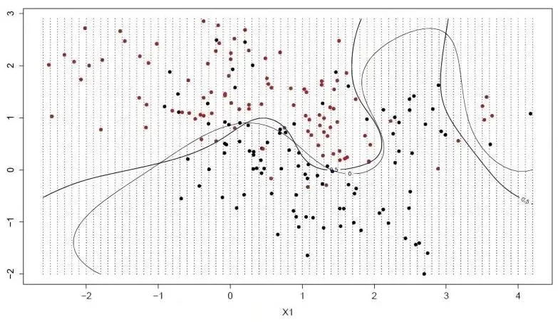
Classification is a very important task in the data mining field. It aims to learn a classification function or classification model (called a classifier). The support vector machine (SVM) is perhaps one of the most popular and discussed classification learning algorithms, which is a supervised learning model and is mainly used to solve the problem of data classification. The SVM is usually used for binary classification problems. It can break down the multivariate classification into multiple binary classification problems before proceeding to the classification. SVM shows many unique advantages in solving issues such as small sample sizes and nonlinear and high-dimensional pattern recognition, and thus is widely used in statistical classification and regression analysis.
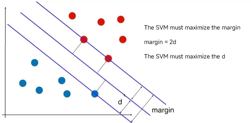
In SVM, a hyperplane is selected to separate the points in the input variable space according to their class (class 0 or class 1), where the hyperplane is the surface that divides the input variable space, which can be regarded as a line in two dimensions, and all the input points can be completely separated by this line. The SVM learning algorithm is to find the coefficients that allow the hyperplane to have an optimal separation of the categories.

The distance between the hyperplane and the nearest data points is called the margin, and the hyperplane with the largest margin is the best choice. Also, only these close data points are relevant to the definition of the hyperplane and the construction of the classifier. These points are called support vectors. They support or define the hyperplane. In practice, we use an optimization algorithm to find the coefficient values that maximize the boundary.
The linearly differentiable support vector machine solution issue can actually be transformed into an optimization solution issue with constraints:

Recall analytic geometry, the distance from a point to a line

Distance from (x, y) to Ax + By +C = 0
Expand to n-dimensional space

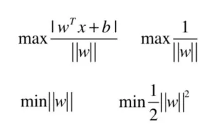
Thus, the final result is transformed into finding the coefficient value corresponding to the following extreme values:

The idea of SVM algorithm classification is very simple, that is, to maximize the interval between the sample and the decision surface with a good classification effect; the final decision function of SVM is determined by only a few support vectors, where the complexity of the computation depends on the number of support vectors rather than the dimension of the sample space, which in a sense avoids the "dimensionality catastrophe". However, it is difficult to implement for large-scale training samples, and it is difficult to solve multi-classification problems with SVM.
4. Random Forest: Improving Biomarker Screening with Ensemble Learning
Random forest (RF) is an algorithm that integrates multiple trees through the idea of ensemble learning. Its basic unit is the decision tree, and its essence belongs to a major branch of machine learning - the ensemble learning method. Random forest, as the name suggests, is a forest that is built in a randomized way. There are many decision trees that make up the forest, and there is no correlation between each of the decision trees in a random forest. After getting the forest, when a new input sample enters, each decision tree in the forest will make a judgment. For the classification algorithm, it will determine which class the sample should belong to. As to which class has been selected the most, this sample is predicted to be in that class. For a regression question, the mean of the k models is computed as the final result.
The specific steps of the algorithm are as follows:
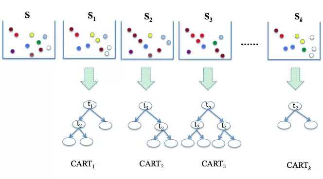
1. First, k training sample sets are drawn from the original sample set S by the bootstrap method. In general, the sample size of each training set is the same as that of S.
2. Second, CART learning is performed on the k training sets, by which k decision tree models are generated. In the process of generating decision trees, it is assumed that there are a total of M feature vectors, and m feature vectors are randomly selected from the M feature vectors. Each internal node is split by utilizing the optimal splitting method on these m feature variables. The value of m is an invariable constant in the process of the formation of the random forest model;
3. Finally, the results of the k decision trees are combined to form the final result. For the classification question, the combination method is called simple majority voting; for the regression question, the combination method is called simple averaging.

The random forest model has many advantages:
1. Excellent accuracy among all current algorithms;
2. Can be effectively applied to large datasets;
3. Can handle high-dimensional input samples without dimensionality reduction;
4. The ability to obtain good results in case of default value problems;
5. The ability to assess the importance of individual features in classification.
Metabolic biomarker screening, i.e., importance assessment of metabolic characteristics, can be performed by random forest analysis. The concept is relatively simple - the main principle is to find out how much each metabolite feature contributes to each tree in a random forest and then take the average value, where the contribution is usually measured using the Gini index or the out-of-band data (OOB) error rate as an evaluation metric.
Finally, a fraction of metabolites with high contribution are selected and used to reconstruct the random forest model for classification.
Next-Generation Omics Solutions:
Proteomics & Metabolomics
Ready to get started? Submit your inquiry or contact us at support-global@metwarebio.com.


