Data Analysis in Metabolomics Biomarker Research-Biomarker Evaluation

1. Unlocking Biomarkers: A Guide to Vital Health Indicators

2. Metabolomics and Biomarkers: Unveiling the Secrets of Biological Signatures

3. Choosing the Right Study Design for Metabolomics Biomarker Discover

4. Metabolomics Biomarker Screening Process

5. Identifying the Right Samples: A Guide to Metabolomics Biomarker Research

6. Data Normalization in Metabolomics Biomarker Research

7. Data Cleaning in Metabolomics Biomarker Research

8. Data Analysis in Metabolomics Biomarker Research

9. Unveiling Biomarkers: Differential Metabolite Screening in Metabolomics Research

10. Data Analysis in Metabolomics Biomarker Research-Biomarker Screening

Welcome back to our in-depth series on metabolomics biomarker research. In our recent posts, we discussed the meticulous process of screening for biomarkers, where we identified and selected metabolites with the highest potential to serve as reliable indicators of biological states or conditions. This crucial step has laid the groundwork for pinpointing candidates that could significantly impact diagnostic and therapeutic strategies.

With our potential biomarkers now identified, the next critical phase is evaluating their performance. Biomarker performance evaluation is essential to determine their reliability, sensitivity, and specificity in clinical or research settings. This involves rigorous testing and validation to ensure that the selected biomarkers can consistently and accurately reflect the biological processes or conditions they are intended to indicate.

In the upcoming blog, we will delve into the methodologies for biomarker performance evaluation. We will explore the criteria and statistical measures used to assess the effectiveness of our biomarkers, ensuring they meet the stringent requirements necessary for practical application.

1. Understanding ROC Curves in Metabolomics Biomarker Evaluation

The ROC curve is a quantitative method that requires experimenters, professional diagnosticians, and those working on predictions to make fine judgments or accurate decisions regarding two conditions or natural states that may or will be confusing. The ROC curve method has been widely used in the medical field for clinical diagnosis and treatment, population screening, and other studies. In metabolomics research, ROC curves are often used to evaluate the diagnostic efficacy of biomarkers.

We need to understand a few concepts first for a better understanding of ROC. When we use a certain diagnostic method to predict a dichotomous outcome scenario, the following confusion matrix is generated:

Sensitivity: it is the ratio of the number of positive cases detected within the group of confirmed diseased cases, i.e., the true positive rate of this diagnostic test. The higher the sensitivity, the lower the chance of a missed diagnosis, i.e., sensitivity = a/(a+c).

Specificity: it is the ratio of the number of negative cases detected within the group of confirmed disease-free cases, i.e., the true negative rate of this diagnostic test. The higher the specificity, the lower the chance of false diagnosis, i.e., specificity = d/(b+d).

Diagnostic accuracy: it is the ratio of the sum of the number of true positive and true negative cases diagnosed to the total number of people tested, i.e., it is the accuracy of the present clinical laboratory diagnosis. That is: accuracy = (a+d)/(a+b+c+d).

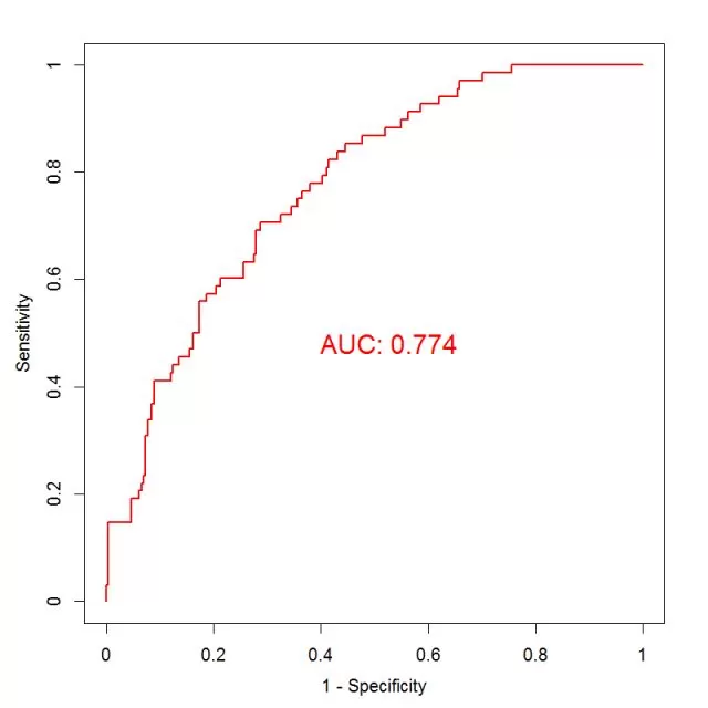
In a diagnostic test, if the test indicator is a continuous variable, a threshold value is typically set, above which it is defined as positive and below which it is defined as negative. When there is no recognized threshold value for an indicator, we can set different values as thresholds, each of which yields a pair of sensitivity and specificity. We plot sensitivity as the vertical coordinate, 1- specificity as the horizontal coordinate, mark the corresponding points of the two in the first quadrant, and connect them with a broken line (as shown below), which is the ROC curve.

The range of the axes of a ROC curve is [0, 1]. The greater the sensitivity and specificity, the better, which means the curve is better the more to the upper left corner. In order to evaluate the diagnostic ability of the indicator, we calculate the area under the curve (AUC), which is the area between the ROC curve and the axes, also known as the C-statistic (area under the curve in logistic regression models: AUC = C - Statistics). The larger the area, the higher the diagnostic power of the indicator. The AUC takes values in the range [0.5, 1] - it's less accurate in the range 0.5 - 0.7, moderately accurate in the range 0.7 - 0.9, and very accurate in the range above 0.9.

We can also find the optimal threshold by curve sensitivity and specificity. In practice, one would like to find the point where both sensitivity and specificity are close to "1". The horizontal axis is (1 - specificity), so the origin of the horizontal axis is the point where the specificity is 1. Therefore, we are looking for the point closest to the upper left corner of the ROC curve, which is the point where the value of (sensitivity + specificity) is the largest. If the importance of sensitivity is considered to be times that of specificity, then the point with the largest value of (a*sensitivity+1*specificity) can be selected. In practice, the threshold can be determined according to different research objectives. If the purpose of the diagnostic test is to screen for the disease, it is advisable to choose a cut-off point with higher sensitivity within the range allowed by the misdiagnosis rate, where a low missed diagnosis rate is ensured. If the purpose of the test is to confirm the diagnosis of the disease, it is advisable to choose a cut-off point with higher specificity within the range allowed by the missed diagnosis rate, where a low false diagnosis rate is ensured.

2. Exploring C-index for Biomarker Performance in Metabolomics

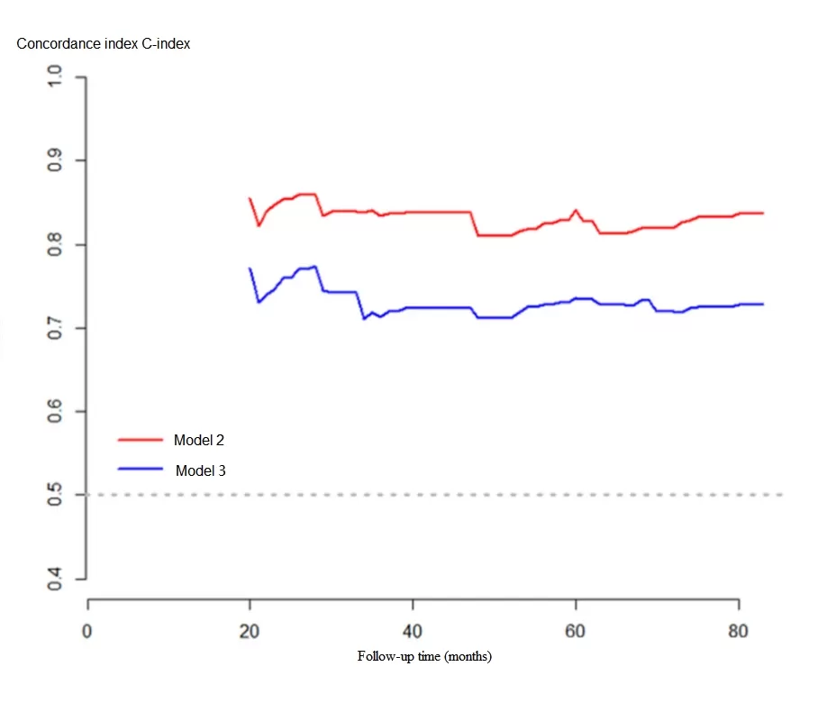
The C-index is also known as the concordance index. It was first proposed by Frank E. Harrell Jr., professor of biostatistics at Vanderbilt University, in 1996. It is mainly used to calculate the differentiation between the predicted value of the COX model and the true value in survival analysis. It is also often used in evaluating the prediction accuracy of patient prognosis models.

The C-index is calculated by randomly pairing all study subjects in the data under study. Taking survival analysis as an example, in a pair of patients, if one of the two with a longer survival time has a longer predicted survival time than the other or if one of the two with a higher predicted survival probability has a longer survival time than the other, then the predicted result is described as being in line with the actual result, and it is called being concordant.

The calculation steps are:

(1) Generate all case pairs. If there are n individuals to be observed, then the number of all pairs should be Cn2 (the number of combinations).

(2) The following two types of pairs are excluded: 1) pairs in which the individual with the shorter observation time does not reach the observation endpoint; 2) pairs in which neither individual reaches the observation endpoint. The remaining pairs are considered useful pairs.

(3) The number of useful pairs in which the predicted outcome is consistent with the actual outcome (concordant pairs) is calculated, i.e., the actual observation time of the individual with the worse predicted outcome is shorter.

(4) Calculate C-index = number of concordant pairs/number of useful pairs.

As can be derived from the above calculation, the C-index is between 0.5 and 1 (the probability that concordance and discordance in any randomized pairwise case is exactly 0.5). Here, 0.5 means completely discordant, indicating that the model has no predictive power, while 1 means completely concordant, indicating that the predictions of the model are completely consistent with the actual situations. In general, a C-index between 0.50 and 0.70 is considered to be of low accuracy; between 0.71 and 0.90 is considered to be of moderate accuracy; and above 0.90 is considered to be of high accuracy.

The C-index is a metric that can be used to determine the discriminating power of various models. For binary logistic regression models, the C-index can be simplified as the predicted probability of developing a disease for patients with that disease is greater than the predicted probability of developing the disease for controls. It has been proven that the C-index for a binary model is equivalent to the area under the ROC curve (AUC). The AUC mainly reflects the prediction capability of binary logistic regression models, but the C-index can evaluate the accuracy of the prediction results of various models, which can be interpreted simply in this way: the C-index is an extension of the AUC, and the AUC is a special case of the C-index.

3. Survival Curves in Metabolomics: Evaluating Biomarker Impact

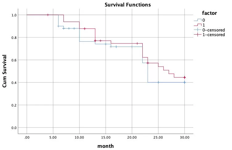
Survival rate is the chance that each individual within a population will survive after a certain period of time. If we take the horizontal axis as the time passed (days, months, or years) and the vertical axis as the survival rate, we can plot a survival curve. The survival curve (also known as the Kaplan-Meier curve) is most commonly used in clinical settings or in life sciences to describe the survival of groups of patients or groups of experimental animals.

The survival curve visualizes the relationship between variable factors and survival and can be used to assess the usefulness of the biomarker. This is done by dividing the samples into high-expression and low-expression groups, respectively, according to the determined biomarker thresholds, and then performing survival analysis. The algorithm is as follows:

Survival rate at a time point = survival rate at the previous time point * (number of individuals that do survive at the current time point/number of individuals that might survive at the current time point) = survival rate at the previous time point * (number of individuals that survive at the current time point / (number of individuals that survive at the current time point + number of individuals that are censored))

It will be easy to understand by giving an example.

Assume that there are 100 patients with the following endpoint events and censored data. Their cumulative survival is calculated this way:

(1) The survival rate is calculated at each time point at which a death event occurs;

(2) A small vertical line is drawn to mark the censored sample at each time point where the censoring occurs;

(3) Plot in groups based on observation/control conditions.

An example is as follows:

4. Odd ratio/hazard ratio: Key Metrics for Biomarker Research

4.1 Odd ratio

The odd ratio (OR) is used to reflect differences in exposure between patients and controls, thereby establishing a link between the disease and the exposure factor. It is usually the ratio of the number of exposed persons to the number of non-exposed persons in the case group divided by the ratio of the number of exposed persons to the number of non-exposed persons in the control group. The formula for calculating OR: [OR = (number of exposed persons in the case group/number of non-exposed persons) / (number of exposed persons in the control group/number of non-exposed persons)].

Example: A doctor suspected that smoking was related to lung cancer because he realized that many of the lung cancer patients he handled had a history of smoking. So he sought out 100 lung cancer patients and 100 healthy controls in 2015 and went back over their smoking histories over the past 30 years. He found that 90 out of 100 lung cancer patients had a history of smoking, while just 20 out of 100 healthy individuals had a history of smoking. This is shown in the table below:

In this case, the ratio of the number of exposed persons to the number of non-exposed persons in the lung cancer group was 9 (90/10); in the healthy individuals, the ratio of the number of exposed persons to the number of non-exposed persons was 0.25 (20/80). Therefore, the OR is 9/0.25 = 36.

The formula in the table is OR=ad/bc.

When evaluating the performance of a metabolomics biomarker, the exposure factor is the content of the biomarker. For example, if tryptophan is screened as a diagnostic biomarker by a disease model, the four-cell table transforms as follows:

The larger the OR value, the greater the effect of exposure and the stronger the correlation between the exposure and the outcome. An OR = 1 indicates that there is no correlation between the exposure factor and the disease; an OR > 1 indicates that the exposure factor is positively correlated with the disease (risk factor); and an OR < 1 indicates that the exposure factor is negatively correlated with the disease (protective factor).

The aforementioned OR is derived from a four-cell table, i.e., only one exposure factor (smoking) was considered in relation to the outcome event (lung cancer). In reality, the occurrence of a disease is often not the result of a single factor. For example, we could assume that smokers are not very fond of fruits and that too little fruit intake could lead to lung cancer. As a result, there is a high probability of an extreme situation where smoking is not associated with lung cancer, and the only reason we have observed an association between smoking and lung cancer in cohort or case-control studies is because of "fruit consumption". At this point, we refer to "fruit consumption" as a "confounding factor", meaning that they may interfere with the relationship between the exposure factor and the outcome variable. In order to eliminate the interference from confounding factors, it is necessary to make some statistical corrections. The most commonly used methods are the Cox risk-proportional model and the logistic regression model. The logistic regression model also yields an OR, but it is calculated differently than the OR described above. The OR from a logistic regression can correct for many confounding factors and is, therefore, a multi-factor-corrected OR, whereas the OR from the four-cell table only considers a single factor and can, therefore, be simply interpreted as a single-factor-analyzed OR. When composing a research article, the multi-factor-corrected OR is generally considered to be more reliable.

4.2 Hazard ratio

The hazard ratio (HR) is primarily used for survival analysis in cohort studies and is derived from the Cox proportional-hazards model. The Cox model shares many similarities with logistic regression, and both of them can be used to correct for confounding factors. The HR value can be calculated based on the Cox model, which indicates how many times more likely the exposed group is to develop the disease than the non-exposed group, taking into account the time at which the outcome occurs.

The figure below is a grouped forest plot of Cox regression results (e.g., assessing the effect of multiple categorical variables on two treatment regimens, S-1+Doc and S-1, with the outcome event: the PFS).

Column 1 shows multiple categorical variables.

Columns 2 and 3 represent the basic conditions of the two groups S-1+Doc and S-1: for example, “87/454”, where the former is the number of cases of an event and the latter is the sample size of each group.

Column 4 is a graphical representation of the HR and its confidence intervals, with the vertical line in the middle of the graph being the null line, i.e., HR=1, indicating that there is no statistically significant association between the factor under study and the outcome; each horizontal line is the study's 95% confidence interval, and the small square in the center of the horizontal line (or other graphics can also be used) is the point estimate of the HR value. If the 95% confidence interval horizontal line of a study crosses the vertical null line, it can be concluded that the studied factor is not statistically associated with the outcome; if the horizontal line falls to the left of the null line, it can be concluded that the studied factor favors the occurrence of the outcome; if the horizontal line falls to the right of the null line, it can be concluded that the studied factor is detrimental to the occurrence of the outcome.

Column 5 shows the numerical representations of the HRs and their confidence intervals.

Column 6 lists the P-values from the interaction tests. When analyzed according to the different variables stratified, an insignificant P-value for the interaction indicates that the results are consistent across the different strata and that the results of the article are reliable.

When evaluating the performance of a metabolomic biomarker, an association between this biomarker and the disease can be demonstrated by using any of the OR or HR analyses.